Stochastic Block Model Simulations

This notebook is used to illustrate how the stochastic block model simulations have been prepared for PyGNA.

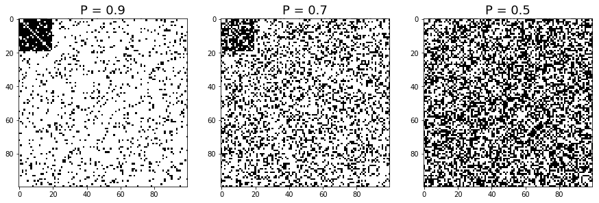
In order to have an understandable figure of the different models, we are going to use different values for the parameters compared to the actual ones. We noticed that on a 1000 nodes network showing different clusters in a 2d representation is very diffult.

Usual representation of a stochastic block model

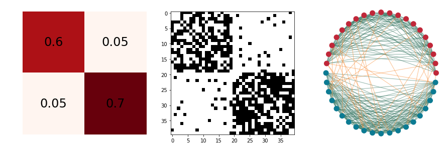
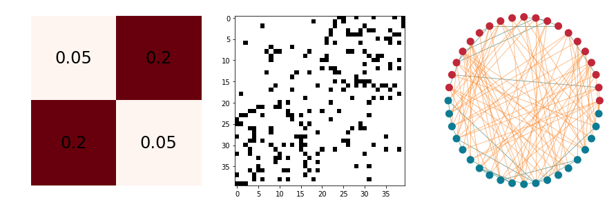
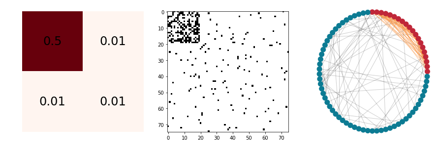
First of all, we show here what the different parameters of a block model represent. In a stochastic block model, the connectivity of the network is defined by the probability of connection of the different nodes. Each node belongs to a block, one parameter, \(p_{ii}\) controls the probability of connection within the i-th cluster while the \(p_{ij}\) parameters control the probability of connection between block i and j.

Here are some examples of a SBM with 2 blocks, each of them with 20 nodes.

For each of the configurations we show: the SBM matrix, the adjacency matrix, and the graph.

We are going to show a strongly assortative network, a strongly disassortative network, and an intermediate case.

PyGNA models

In order to simulate a realistic network, we use the stochastic block model to generate both the whole network and the clusters of intereset.

To do so, we have to define a larger block, whose probability of connection represents the general connectivity of the network, and a smaller block which is going to be the cluster of interest.

All the simulations in PyGNA are done by parametrising the number of nodes in each block and the SMB matrix.

Two clusters SBM

In the simplest model, we parametrise two blocks by varying the number of nodes in each cluster and the SBM matrix.

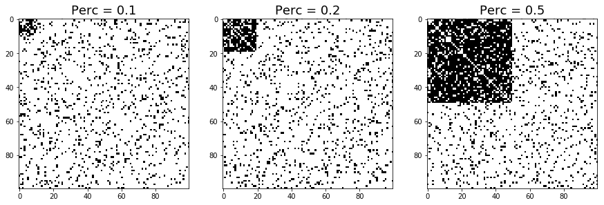
With the parameter \(perc\) we specify the percentage of the total number of nodes that is assigned to the cluster of interest. Instead, the SBM matrix is parametrised by varying \(p_00\) and \(p_{01}=p_{10}=p_{11 = 1-p-{00}}\).

Percentage of nodes

Here is how the adjacency matrix varies with different percentages of nodes in the blocks.

Connection probabilities

Here we show how the adjacency matrix varies for different probabilities of connection.